

The Mechanical Engineering Technical Interview

So, you’ve secured a technical interview!
Ideally, that was the hard part. Now it’s time to dazzle them with your deep understanding of everything engineering. Unless… you haven’t taken those classes yet.
But no worries, you can just Google “mechanical engineering technical interview questions” and go on your merry way.
Except… the resources online for this are terrible. And I mean TERRIBLE. This one enraged us enough to create the very website you’re on now.
The Basic Technical Interview Framework:
Interviewer Introduction
Your interviewer will introduce themselves, say what team they work on, what they do, etc. You should already know all this information. Stalk them on LinkedIn beforehand and learn everything there is to know about them. It’s not creepy, it’s initiative — mentioning their prior research or asking a thoughtful question on what it’s like working at company X vs company Y shows resourcefulness and interest, two of the key ingredients to success during an internship
Elevator Pitch
When you introduce yourself, start off with what year you are, where you’re from, what you’ve been working on at school, etc. Sometimes they will ask you to briefly go over your resume. Elaborate on technical projects, personal contributions, and results. Where did you thrive and what did you like working on? This should be practiced and clean. The interviewer will often ask you a few questions related to things you mention so be prepared to answer (but do NOT violate any NDAs - that can mean researching what is publicly available information or generalizing before the interview). Don’t expect to cover every item on your resume, most likely you will only get through 2-3 experiences/projects, so cover items in order of relevance and significance. First impressions aren’t everything, but a good one certainly can’t hurt.
Technical Time
Though it’s possible that your interviewer will simply ask technical questions related to the projects on your resume as you go through it, it’s more likely they will eventually cut you off and say “Let’s do some technical questions now.” Depending on how long resume coverage takes (contingent on how compelling you are and who’s interviewing you), there could be anywhere between 15 and 40 minutes left at this stage. This is the part where they can ask you any question about anything in the entire world. I have been asked about the unique material property of cork, to name 5 countries in Africa, and anything in between. The less confident you are in your ability to handle this part, the longer you want to spend on your resume/projects. The remainder of this page is dedicated to covering the most common questions an interviewer will ask.
Any Questions?
At the end of every single interview, your interviewer will ask: “Do you have any questions for me?” The answer to that question should always be: “Yes!” This part of the interview is critical to making sure you stand out. Research the company before your interview, and prepare these questions ahead of time. I generally have a list of questions written down (though you will likely only ask 2-3 of them). These aren’t just any run-of-the-mill questions you’re asking. These are deep, well-thought-out questions on subjects like struggles you think the company is having and how they’ve addressed that issue. Do not waste these questions on something like “Is there a transportation stipend?” The interviewer is very unlikely to know or care, and you’ve now portrayed the viewpoint that you are merely looking for money, and not passionate about the mission of the company — this can be a critical oversight, especially within the tech and startup space where the engineers working at a company are likely highly mission-driven.
Cantilever Beams?
After this, it’ll be more like CANilever beams.
Cantilever beams are the fundamental basis of most technical questions you can expect to be asked. It pays dividends to know them backwards and forwards (and across the neutral axis- a little humor that will make sense later if it doesn’t now). More than that, it is highly advisable to understand the why in addition to the answer, as variants to this question are exceedingly common. Materials, equations/intuition, and design considerations can all be covered through this simple object, and understanding of those subjects can rapidly be gauged by the interviewer.
There will be 3 depth levels available to learn at: Need to Know (vital to doing well), Preferred to Know (knowledge expected), and Nice to Know (ace the interview).
Click the link to go to that portion of this very very long page
Need To Know
Free Body Diagrams
Max Beam Deflection
Basic Materials
Loading Conditions
Stress-Strain Curves
Buckling
Nice To Know
Distributed Loading
Basic Inertial Calculations
Cross-Sectional Analysis
Advanced Materials
Strength To Weight Ratio
Heat Treatment
Carbon Content
Grain Structure
Manufacturing
CNC
3D Printing
Injection Molding
Advanced Buckling and Linkages
Effective Length
Design Considerations
Single Shear
Natural Frequency
*Coming In 2024
Free Body Diagrams (FBDs)
This is an imperative tool in any engineer’s arsenal, and something you usually learn in introductory physics.
It is essentially a simplified diagram showing the forces acting on an object.
Let’s break it down.

The most simple case of this is an object in free fall.
For example, a skydiver falling through the air. A skydiver experiences only two forces (for our purposes): drag force (Fd), and force of gravity (Fg). Force of gravity is equal to mass times acceleration due to gravity, or mg.
The drag force equation we can mostly ignore, just know that drag force is proportional to velocity squared (in our simplified example).
The concept of terminal velocity, practically speaking, is the max velocity an object in freefall will reach. This is because drag force increases with velocity until it equals force of gravity (relatively constant).

A slightly more complicated case would be a hockey puck sliding on ice as shown to the left.
We will consider three forces as it slides on the ice: gravity, the normal force, and friction.
Please take a moment here to convince yourself that the normal force has to be equal to the force of gravity in order to prevent the puck from floating into the air or sinking into the ice.
Familiarize yourself with Newton’s second law if this still isn’t clear to you.

Max Beam Deflection
Now let’s tie it all back! To the right is a photo of the legendary simply supported cantilever beam.
The most common question is: if I apply a force F at the end of the beam, in what ways can I minimize the maximum deflection?
There are a few ways to answer this question. One, you could just give the formula: (FL^3)/(3EI) where F is force, L is length, E is a material property, and I is moment of inertia. However, the better way to answer this question is to explain the different variables and why they affect the beam in the way that they do. Essentially, derive the equation qualitatively. Anyone can memorize a few formulas, but understanding of what drives them is what shows intuition and ability to apply that knowledge to new situations.

Basic Materials
Now you’ve arrived at the all-important material selection stage. Materials are a cornerstone of mechanical engineering knowledge and a lot of cool innovations are currently being made in this area for those interested in specializing in it.
Be forewarned, for those without prior background in materials, there is a lot of jargon and most of it is absolutely necessary to be able to use fluently so pay attention to this section in particular.
There are also many, many considerations that should be made here, some more important than others. Most of the time, however, you will not have all the information to make those decisions from a fully informed viewpoint. Thus it can be appropriate to ask questions about the loading condition and environment.
Which axes are loaded? Is load relaxed and repeated frequently? Is this a rainy or snowy region? Is it by the sea or in contact with corrosive chemicals? What is the ambient temperature of the environment? Is weight an issue? Is it manufacturable? What’s the budget? How many need to be created?
Do NOT just memorize and ask some of these questions. Aside from it showing a profound lack of understanding, the most common response to a question is “Why do you ask?” A question is not just an opportunity to learn more, it is an opportunity to engage and show the depth of thought that led you to ask the question.
Above were just a handful of the things that you should be thinking about in the back of your mind. However, the most common (and important) thing to check when designing something to withstand loading tends to be yield strength, a property of the infamous stress-strain curve.
Starting simple, the y-axis is stress and the x-axis is strain. Recall stress = force/area and strain is total elongation/original length. Always focus on understanding the meaning behind the words, anyone can read material properties of a stress-strain curve, but understanding the basics is critical to be able to tell what material it might be, or explain how snapback works, or what it means that the yield and ultimate strength are located near each other.

With that In mind, imagine a pencil-sized rod of aluminum. As I apply tension to each end, the rod stretches ever so slightly. However much force I applied, divided by the initial area, is the stress in the part. The strain is how much it shrinks or grows as a proportion of overall length. Generally speaking, if I use a thicker rod of aluminum, the force/area will result in the same amount of strain. That makes this curve independent of form factor and thus the resulting stress/strain ratio is a material property.
Graphically, this ratio is the slope of the line as long as it remains linear. The value of the slope is also known as Young’s modulus, or the elastic modulus, and is fundamental to basic material analysis as it relates deformation to stress. That linear region of the graph is also called the elastic region. This is because as long as when we apply stress to material and it stays in that elastic region, it will return back to its initial state afterward. In other words, the material will act (unsurprisingly) elastically!
The point at the very top of the elastic region, the point after which the line is no longer linear, is appropriately dubbed the yield strength (YTS = yield tensile strength). If the stress exceeds that value, the part will no longer return to its original state. There will be some level of permanent deformation.
The ultimate strength (UTS = ultimate tensile strength) is correspondingly the max stress the material can undergo (see “Preferred To Know” for the more complicated truth).
When designing different parts, engineers may design to UTS or YTS for different purposes. Localized yielding (determined through simulation) may also be acceptable. It all depends on use case.
For now that’s really all you need to know about stress strain curves, but there is plenty more on it in the other depths.

Buckling
The last thing you absolutely need to know about is buckling. Buckling and yielding are the same in that a part inelastically deforms (or fails to return to its original condition), however, they are very different in that buckling will cause your part to break catastrophically and dangerously while a small amount of localized permanent deformation can be acceptable in certain use cases.
The most common scenario that might come to mind when you think of buckling, is perhaps a knee, buckling to allow impact absorption over a greater distance. A hyper simplistic model of a leg, might consist of a two-linkage system with a joint at the knee. However, for the time being, we will take a look at the simplified one-linkage system.
Linkages are one of the most common components in automotive and aerospace engineering, as they allow for highly effective transfer and distribution of force. Examples I’ve worked with include the pushrod of a suspension and the gimbal of a rocket. Both are relatively simple components, but critical to success.
Doing the buckling calculations properly to ensure no failure occurs is a basic and essential skill that should be in any mechanical design engineer’s toolbox.

Pictured to the right is the most basic buckling problem:
How large can the force F (in red) be before the linkage (in black) buckles?
Another formula to know: Pcr = (π^2*E*I)/(KL)^2
Pcr is the critical load at which the linkage is likely to buckle.
E is young’s modulus, a material property relating stress to strain as explained previously.
I is moment of inertia and is dictated by the cross section of the linkage.
L is the length of the linkage itself.
K is the effective length factor and it will be covered more in the next section. In short, it is a scaling factor that is applied to length depending on the type of connection (rigid, pinned, rolling, etc.)
Look at these variables and understand their place in the equation. If I use a stiffer material, E increases and logically, I would expect it to be more difficult to buckle. If I use a larger diameter tube, inertia increases with the square of radius and it is also expected that this would intuitively cause the tube to be more difficult to buckle. Lastly, the shorter the linkage, the more difficult to buckle. Make special note that decreasing the length will have a magnified effect relative to changing material or cross section as reflected by its square in the equation.
Shear and Moment Diagrams
The standard issue interview question on this topic typically has to do with a street sign / shop sign / stop sign. Whatever it is, it’s essentially a long beam with a force applied at the end or distributed along the length.
A useful tool to graphically represent the forces/moments along the length of the beam are shear and moment diagrams.
If you’ve taken statics (and did well), you can probably skip this section.
The basic idea, is that without understanding what the internal forces are within a component, it is impossible to effectively optimize the design. This means your component will be heavier than it needs to be, cost too much, and/or be weaker than it needs to be. By looking at those internal forces/moments, we can also get an idea of where our component will fail.
To begin with, let us consider a frequently used example, the simply supported beam under uniformly distributed loading (UDL).

When the beam experiences a force (in this case, a distributed one), it will experience stress. If the force is high enough (beyond the yield stress), it may even plastically deform. We are able to examine that stress through representing it as a shear force and a bending moment. The shear force we are examining is along the cross section, while the moment is the result of forces going into and out of the cross section of the beam.
Calculate Reactions
Given:
Beam length = L
Uniformly Distributed Load (UDL) = w (kN/m or lb/ft)
For a simply supported beam with a UDL across its entire span, RA and RB (reactions at supports A and B) are each half of the total load on the beam.
RA = RB = (w * L)/2
*Note that it is conventional to define the positive and negative of shear forces as shown on right.
Also, note that this can sometimes be confusing, and so long as you are consistent in your definition of axes, you will be correct, even if your solutions are [uniformly] off by a negative from whatever the answer key has.

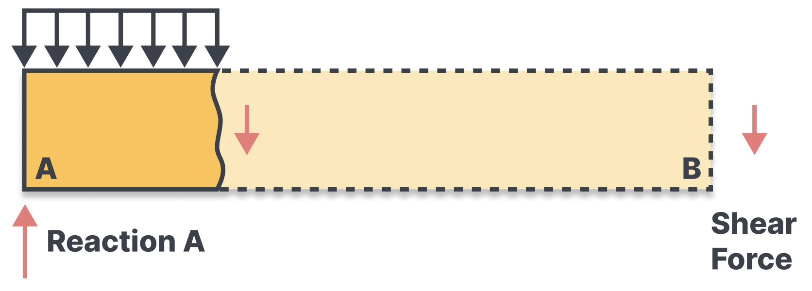
Shear Force Calculation (Method of Sections)
The name of the game here is force balance. Starting from one end (let's say from A), at the very beginning (just to the right of A), the shear force V is equal to RA. Always remember that in statics, the net sum of forces is zero! The beam doesn’t have an acceleration, and it doesn’t fly into space. It is a static structure, so for F=Ma to remain true, there must be another force (or forces) acting oppositely.

As we move along the beam from A towards B, the shear force reduces linearly due to the UDL. For a distance x from A, the shear force V is:
V(x)= RA − w * x
At the midpoint of the beam, the shear force is zero.

As we continue moving from the midpoint towards B, the shear force becomes negative (remember our axes definition from above!) and continues to increase in magnitude (read: get more negative) linearly.
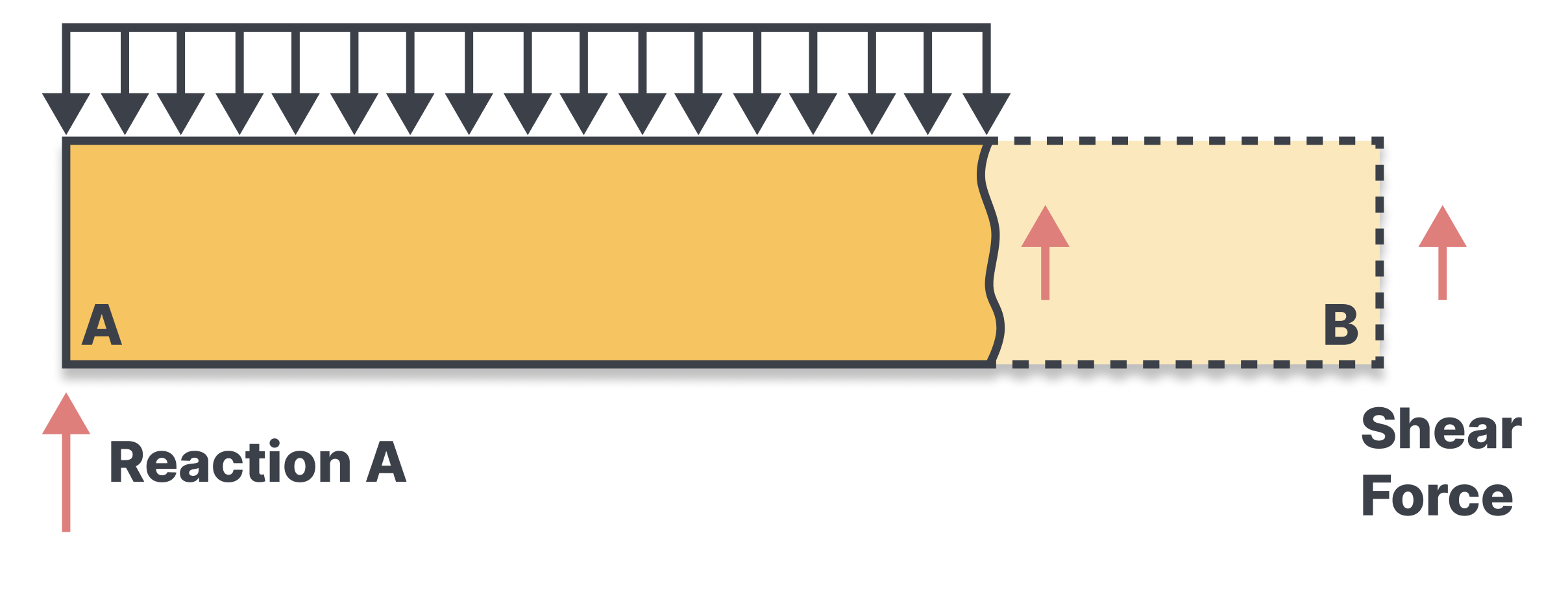
Right before support B, the shear force is −RB.

And finally becomes zero again after the rolling support is reached.

Bending Moment Calculation
At supports A and B, the bending moment M is zero (because they're simple supports, no moment can be applied by definition. Moments applied at a support require rotational constraint). The bending moment increases as we move away from A (or B) and is maximal at the midpoint of the beam. For a distance x from A, the bending moment M is:
M(x) = RA * x − 0.5 * w * x^2

The maximum bending moment at the midpoint is:
Mmax = (w * L^2)/8

As the shear force switches sign past the halfway point, it applies a moment in the opposing direction to the UDL, and the overall moment decreases.

If you’re paying attention, you may be wondering how the equation M(x) was found. The easiest way in most cases, is to integrate the equation for shear force (V(x)) and plug in initial conditions. It’s a very simple integration here so try and prove to yourself the validity of the relationship. To prove the relationship, use a differential element and examine its forces and moments. This is usually unnecessary in interviews though it is generally good knowledge to know in case you need to derive something on the spot.
Beam Breakage
The last thing on shear moment diagrams that is almost certain to be asked, is where the beam breaks if the loading is too high. The answer? Almost always the max bending moment, don’t forget it. Additionally, where on the beam will it break? Usually in tension as most materials better resist compression and ductility works in our favor by slightly increasing area as it bunches up in the compressed area. So, in this example, the beam will most likely break in the middle on the bottom surface. To be more specific, material must be selected as sometimes other failure modes can be limiting in certain materials.
ALRIGHT, let’s apply the knowledge from the question to a fixed end cantilever beam with point loading this time! This exact configuration of beam and loading will come up in about 50% of technical interviews, and most others will at least touch on a variant of it.
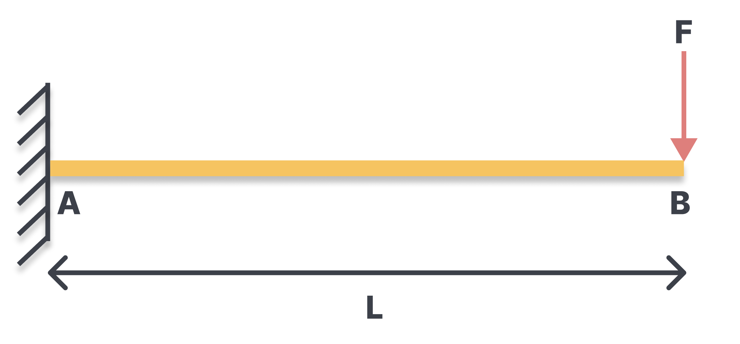
The vertical reaction at the fixed end (RA) is equal to P as it must counterbalance the load to maintain vertical equilibrium. In addition to the vertical force, the fixed end will also experience a moment due to this point load. The moment reaction at the fixed end (MA) is P * L.
Shear force diagram: Beginning from the fixed end, and moving right towards the free end (x = 0→L), the shear force value remains constant at RY = P across the entire length of the beam.
Note that shear force remains positive despite being pointed in the negative Y direction due to the shear force orientations we have chosen as negative and positive above. Consistency here is key!
Shear force (x) = P

Bending moment diagram: Starting at the fixed end, the moment is solely composed of -MA = -P * L. As we move towards the free end, a factor of P * d is added (given it is an applied moment in the opposite direction) due to the shear force. When we each d = L, the added factor = P * L = MA, making our overall moment 0.
Moment (x) = -P * L + P * x = P * (x - L)

Cross Section
Another important and related topic examines the cross section of the beam. For these simple problems, it is intuitively very easy to figure out where the beam is in tension and where it is in compression (simply allow the beam to bend in your mind and see which part gets longer vs shorter). However, intuition only gets us so far for more advanced setups, so a graphical approach is also needed.
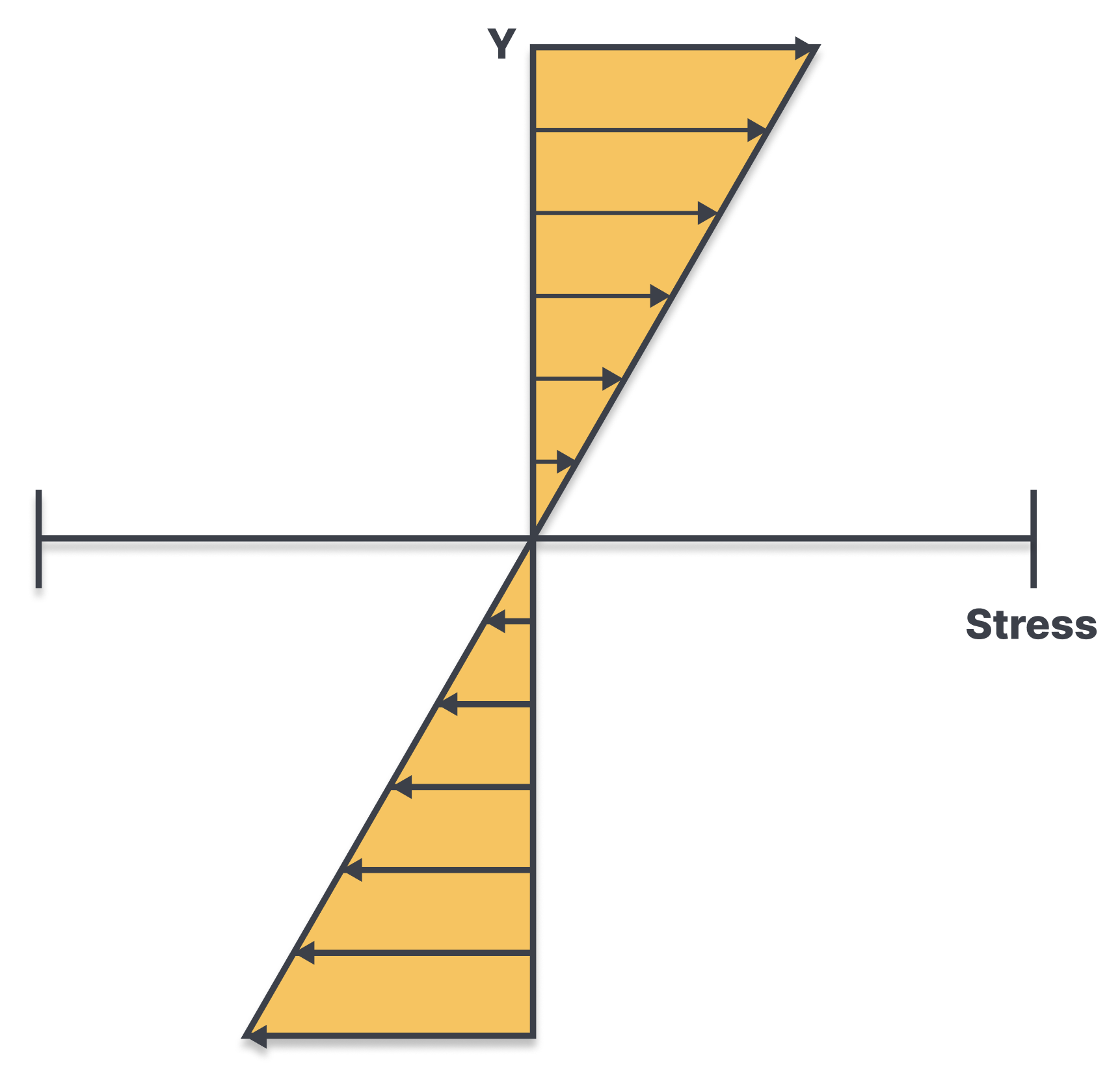
At the heart of this graphical approach lies the concept of the neutral axis. When a beam bends due to the application of external loads, there's a particular plane within the beam that neither elongates nor compresses. This plane is termed the "neutral axis." Above this axis, the beam material is in compression, and below it, the material is in tension.
The position of the neutral axis is closely tied to the geometric properties of the beam's cross-section, specifically its centroid or center of gravity. For symmetrical sections like a rectangle or a circle, the neutral axis lies at the geometric center. For unsymmetrical sections, its position may differ, but it can be determined through calculations related to the section's centroid.
For this case, our graph shows no stress along the neutral axis, tension above it, and compression below it. This makes logical sense and is very easy to come up with. If another load is added to our beam, it may be difficult to visualize intuitively. Luckily, the graph for an alternate loading scheme can be determined, and superimposed onto (added to) this graph. Try adding a compressive force at the free end and see how the neutral axis actually shifts! This can be very useful for optimizing beam designs to support the area with the most stress.
So how can we optimize/evaluate the beam shape? As you might’ve guessed based on the name of this section, inertia! Inertial analysis begins with finding the centroid of an object as that dictates the neutral axis. Thinking of the centroid as the center of mass (even though we’re looking at a 2D cross section - so more of a center of areas then) can often make it relatively easy to find given many simple shapes are symmetrical. For example, a standard rectangle has its centroid in the center and inertia = (1/12)bh^3. A triangle or other shape centroids can be found by integrating in the proper direction (integrate x to find Cx and y to find Cy) and dividing by A. This finds the average point across the area in that direction. Inertial equations can be derived based on integrating a differential element, but that is rarely expected in an interview. I instead recommend memorizing the inertias and centroids of a few key shapes, or buying our interview cheat sheet to help with prep. The most common one which you absolutely need to know is the inertia of a rectangle = (1/12)bh^3.
So now that we know the inertia of rectangle, how can I find the inertia of an I-beam? A beautiful little theorem called the parallel axis theorem. This theorem allows us to simply add together inertial contributions from different components based off of distance to the centroid.

To find the moment of inertia of an I-beam using the parallel axis theorem, it's useful to first break down the I-beam into simpler geometric shapes. An I-beam can be divided into three rectangles: one rectangle at the bottom, one in the middle, and one at the top. These three rectangles are aligned along their centroids. Let's say the bottom and top rectangles each have a width b and a height t, and the middle rectangle has a width w and a height h.
The parallel axis theorem states that the moment of inertia of a shape about any axis parallel to and a distance d away from an axis through its centroid is I = Icentroid + Ad^*2, where Icentroid is the moment of inertia about the centroidal axis, A is the area, and d is the distance between the two parallel axes. Simply put, based off the area and distance from the centroidal axis, we can use superposition to add in a corrective factor to the inertia!
First, we find the moment of inertia for each of the three rectangles about their own centroidal axes:
For the bottom and top rectangles: Irect = (1/12)*bt^*3
For the middle rectangle: Imiddle = (1/12)wh^3
Next, we calculate the area for each of the three rectangles:
Area of either the bottom or the top rectangle: Arect=bt*
Area of the middle rectangle: Amiddle=wh*
Now we find the distance d from each rectangle's centroid to the centroid of the entire I-beam. The centroid of the I-beam is located at the midpoint along its height H, where H=h+2t.

Ibottom=(1/12)bt^3+bt×dbottom^2
Itop=(1/12)bt^3+bt×dtop^2
Imiddle=(1/12)*wh^*3+0 (since dmiddle=0)
Finally, the moment of inertia of the entire I-beam about its centroidal axis is the sum of the moments of inertia of these three rectangles:
I-beam=Ibottom+Itop+Imiddle
Note that you usually won’t have to actually apply the parallel axis theorem in an interview. Instead, simply use it to explain why material further away from the neutral axis (centroid) has a greater effect than material closer (added inertia scales with d^2).
A very common interview question is to compare several beams and say which one is the best for a certain application. Using your knowledge of inertial calculations, shear moment and cross section diagrams you should be properly equipped to optimize beam sections and evaluate their effectiveness. Just be sure to take a step back and think, there are also some common trick questions in this domain (which we cover in our technical interview book).
Intermediate Materials
Understanding of materials is crucial to success in most technical interviews for MechE positions (especially PD or simulation roles). One of the easiest topics to cover (and one which is almost certain to come up) is stress strain diagrams. One of the classic questions here is to draw and compare the stress strain diagrams for five different materials, usually aluminum, steel, ceramic, rubber, and plastic (PP = polypropylene or something similar). They may also just ask about aluminum and steel depending on how badly they want to grill you.
Assuming you’ve already read our beginners guide or taken an intro materials course, you should already know all about yield strength, ultimate strength, necking, and fracture. There are two other things you can very reasonably be expected to know: true vs. engineering stress, and snapback.
True vs Engineering Stress

The gist of true vs. engineering stress, is that as the tensile sample (also frequently called a “dogbone” for obvious reasons) is strained, assuming it has a standard poisson’s ratio, due to conservation of mass the cross section will reduce in area. In typical stress strain graph generation, we only measure the initial cross section, and all stresses are computed based off that value. That is why the ultimate stress shows up as a local maxima! It’s not that the material actually gets weaker after that point, it’s that the cross section has reduced so much that the material appears to get weaker from a macro scale! In a true stress strain curve, area is recalculated at each point on the curve to provide a true stress. In practice, this is annoying and usually somewhat pointless except in critical applications. For that reason, given that engineering stress always provides a more conservative estimate of strength, engineering stress is often used! More info on this can be found in our interview book!
Note: For info on non standard poisson ratios, read up on auxetic materials. Fair warning, I’ve only been asked about this once and it was exceptionally cruel of the interviewer.
Strain Hardening
Snapback or Strain Hardening is the phenomenon where, when a material is stressed above the yield limit, then allowed to relax back to a neutral state, the curve shifts!

As the material is released in the strain hardening region (plastic deformation), some amount of energy has gone into plastically deforming the material. When released, it will no longer spring back to its initial state (per the definition of yield stress). Instead, it will travel back following the slope of Young’s modulus. Where it lands on the x axis can be used to determine the amount of permanent deformation the material has sustained. The integral of the region between the two curves, is the amount of energy that went into that permanent deformation. It is crucial to remember here, that after yield stress, not all strain is inelastic. Any further strain has both an elastic component, and an inelastic component. This is why, when released from a higher stress, the elastic region appears to grow. Such a concept can easily be integrated into our cantilever beam question by asking to show on the stress strain graph what will happen to the beam after released from a load
Fatigue Curves
When FEA results show localized yielding, it is often ignored in low cycle parts. This is because slight yielding (below ultimate stress) will result in only very minor changes to geometry given that the material will snapback to a pseudo-initial state. If extended to a high cycle part, this could pose a problem due to crack propagation or fatigue at the relevant site.
Speaking of fatigue, SN curves are another curve which you should be familiar with prior to going into an interview.
What is an SN curve? Essentially, they are best fit curves generated from a sweep of data where varying loads are applied (and corresponding stresses induced), and the number of cycles sustained before failure is measured. It’s called “SN” (pronounced ESS-EN) because Stress is on the Y axis, and Number of cycles is on the X axis, though it should really be called N(S) because technically the stress is the independent variable in the plot generation. Be sure to note the log scale of the axes.
Most SN curves appear to face some form of asymptotic decay. This belies the existence of what is termed, “the endurance limit.” The endurance limit is an amount of stress, less than which a material can theoretically be brought to an infinite amount of times without experiencing failure.

Notably, not all materials possess a distinct endurance limit. Materials like aluminum do not exhibit a well-defined endurance limit; their S-N curves continue to descend, suggesting an ever-present risk of fatigue failure, however low the stress may be. Anyone who has ever ripped apart a soda or beer can after twisting it back and forth a couple times has experienced aluminum’s poor performance in fatigue. Given the prevalence of aluminum due to its weight and cost, this is an important detail for engineers to remember, always considering the number of cyclic loadings which our parts will undergo.

Being able to explain the difference between aluminum and steel in fatigue is frequently helpful in technical interviews, though the interviewer may not be as direct as asking about the SN curve. Instead, they are likely to ask you questions alluding to fatigue after assigning a material. It is then your responsibility to bring up the endurance limit (or lack thereof) and explain the relevant SN curves.
As a rule of thumb (generally not accepted as having a high degree of accuracy), cyclic load cases can be superimposed on one another to mimic a use profile under Miner’s Rule. Formally, Miner's Rule is a linear damage accumulation model used to predict the fatigue life of a structure subjected to varying stress levels. According to this rule, the total damage D at any point in time is the sum of the fractional damages at various stress levels:
D=(1—>n)∑Ni/Nf,i
Here Ni is the number of cycles experienced at stress level i, and f,Nf,i is the number of cycles to failure at the same stress level as per the S-N curve. When D reaches or exceeds 1, failure is expected.
A more intuitive way of looking at the rule, is that there is a finite fatigue “life” of a material, similar to health points (HP) in a videogame. Any point on the curve will take 100% of the HP of our material (we expect it to fail at that point). However, any point below the curve will take some fraction of the material’s fatigue life. If that material experiences multiple, different cyclic loadings, those fractions can then be added up to figure out whether or not we expect the material to fail.
Running through a relevant example, let’s consider a fixed-end cantilever beam subjected to three different types of cyclic loading: low-level, medium-level, and high-level stresses. The aim is to predict the beam's fatigue life using Miner's Rule, leveraging the S-N curve data for the material.
Assumptions:
The material's S-N curve is known.
The low-level stress will have an amplitude of 50 MPa and will be applied for 1,000,000 cycles.
The medium-level stress will have an amplitude of 100 MPa and will be applied for 500,000 cycles.
The high-level stress will have an amplitude of 150 MPa and will be applied for 100,000 cycles.
S-N Curve Data:
At 50 MPa, the material can withstand 2,000,000 cycles before failure (Nf1).
At 100 MPa, the material can withstand 1,000,000 cycles before failure (Nf2).
At 150 MPa, the material can withstand 250,000 cycles before failure (Nf3).